Tutorial

Initiate a Geometric_Brain_Network object

Create a simplicial ring complex on a ring. Topology is only available for a ring now. GD, geometric degree, is the local neighbors of a neurons whereas nGD, nongeometric degree, is the distant neighbors of a neuron.

#### NETWORK VARIABLES
size = 400
GD = 10
nGD = 4
topology = 'Ring'
noise = 'k-Regular'
network = Geometric_Brain_Network.Geometric_Brain_Network(size, geometric_degree = GD, nongeometric_degree = nGD, manifold = topology, noise_type = noise)

Inheriting neuron objects

Define neuronal properties and then use get_neurons to inherit individual neurons into the network.

    #### EXPERIMENT VARIABLES
TIME = 100 ## number of iterations
seed = int(size/2) ## seed node
C = 10000 ## constant for tuning stochasticity(high C yields deterministic experiments)
K = 0 ## constant weighing the edges vs triangles K=0 pure edge contagions, K=1 pure triangle contagion

#NEURON VARIABLES
threshold = 0.2 # node threshold
memory = TIME ##When a node is activated, it stays active forever(SI model) when memory = TIME.
rest = 0# neurons don't rest

##INITIATE NEURONS and Inherit them
neurons = [Geometric_Brain_Network.neuron(i, memory = memory, rest = rest, threshold = threshold) for i in range(size)]
network.get_neurons(neurons)## this is for runnning experiments with new set of neurons without changing the network

Run a single example cascade

Core function run_dynamic runs an experiment with given variables.

activation1, Q1 = BN.run_dynamic(seed, TIME, C, K)

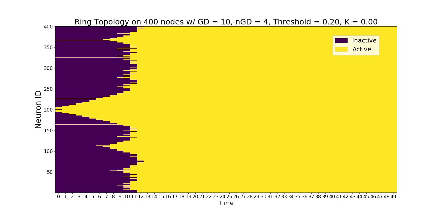
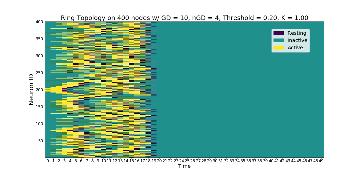
A single experiment starting at the seed node 200. Initial wavefront propagation can be observed.

Running experiments without changing the network connectivity

One may want to work with a different set of experiment or neuronal variables without changing the underlying topology. This is when get_neurons function comes handy.

## with a new set of variables you can run a new experiment without changing the network
K = 0
threshold = 0.3
memory = TIME
rest = 0

neurons_2 = [neuron(i, memory = memory, rest = rest, threshold = threshold) for i in range(size)]
BN.get_neurons(neurons_2)

activation2, Q2 = BN.run_dynamic(seed, TIME, C, K)

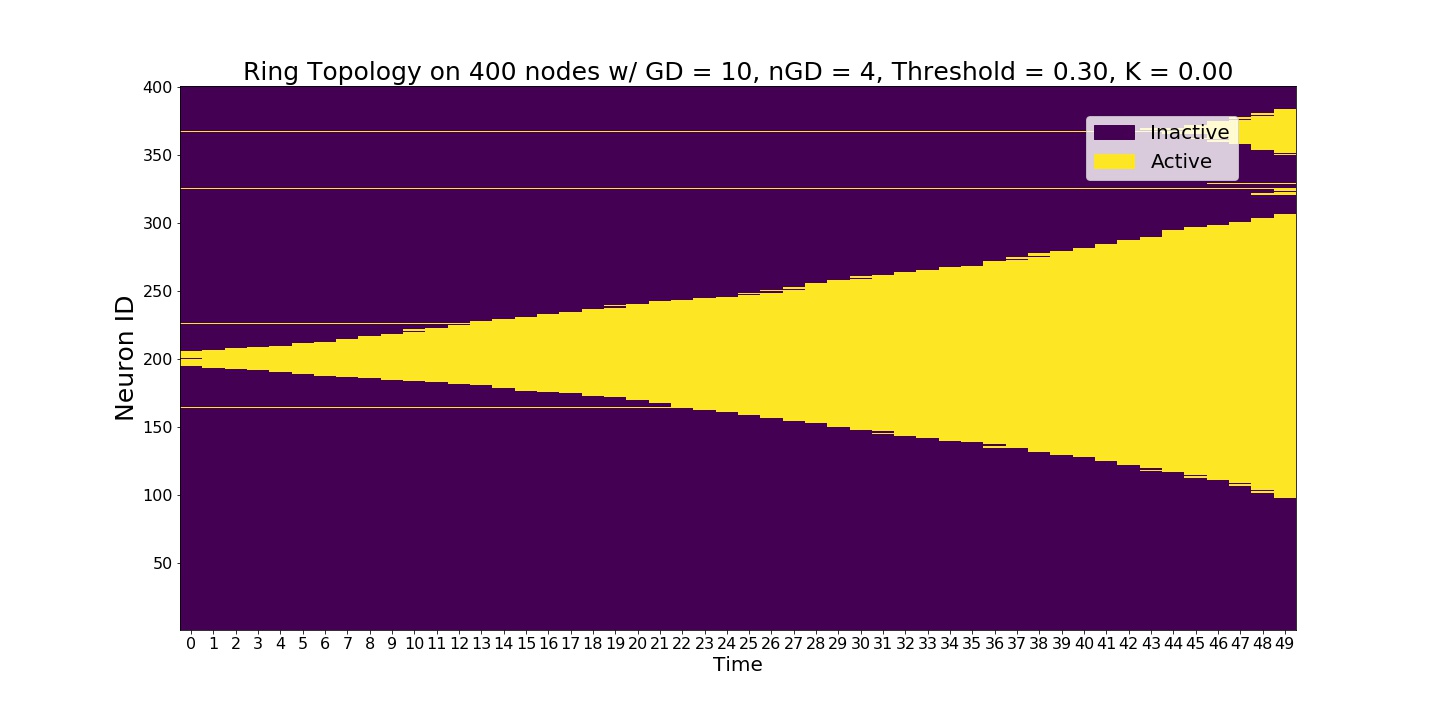
We increased the global node thresholds to 0.3 which slowed down the signal, wavefront.

Running simplicial cascades

Simplicial cascades can be ran by simply varying the parameter \(K\) between 0 and 1.

## with a new set of variables you can run a new experiment without changing the network
K = 1
threshold = 0.2
memory = TIME
rest = 0

neurons_3 = [neuron(i, memory = memory, rest = rest, threshold = threshold) for i in range(size)]
BN.get_neurons(neurons_3)

activation3, Q3 = BN.run_dynamic(seed, TIME, C, K)

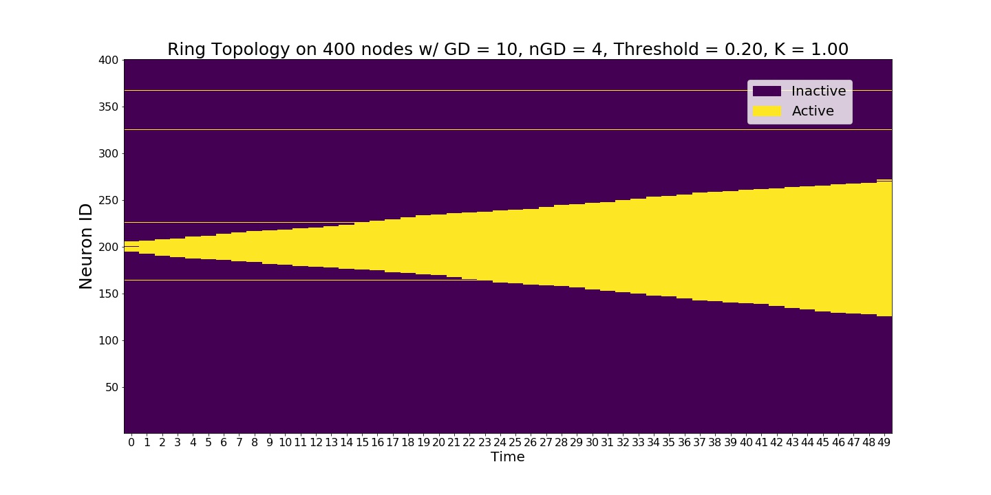
Even though the global node threshold is 0.2 we observe a slow signal. The reason is that we set K=1 which implies a full triangle contagion.

Neurons with memory and refractory period

Our model is as general as it can be. So, neurons can have arbitrary number of memory or refractory period given in discrete time steps. This generalization increases complexity of the dynamics really quick.

K = 0.5 # average of edge and triangle contagions
memory = 1## memory of a neuron is how many time steps neurons are going to stay active after they activated once
rest = 0#rest of a neuron is how many time steps neurons are going to be silent after they run out of memory, refractory period.
threshold = 0.2

neurons_4 = [neuron(i, memory = memory, rest = rest, threshold = threshold) for i in range(size)]

BN.get_neurons(neurons_4)

activation4, Q4 = BN.run_dynamic(seed, TIME, C, K)

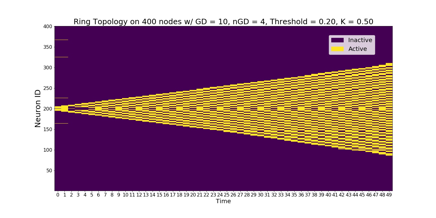
Slow signal propagation where neurons are active only 1 time step. Signal spreads as the neurons blink.

Running stochastic models

Stochasticity of the neuronal responses can be adjusted using the experiment variable \(C\). Higher values make the system deterministic.

K = 1 ## triangle contagion
memory = 2## memory of a neuron is how many time steps neurons are going to stay active after they activated once
rest = 1#rest of a neuron is how many time steps neurons are going to be silent after they run out of memory, refractory period.
threshold = 0.2
C = 10 ## make the system stochastic, higher values(C>500) is going to make the system deterministic

neurons_5 = [neuron(i, memory = memory, rest = rest, threshold = threshold) for i in range(size)]

BN.get_neurons(neurons_5)

activation5, Q5 = BN.run_dynamic(seed, TIME, C, K)

As the refractory period is nonzero, complexity of the system increases exponentially.

Looking at the cascade size

We can plot the size of the active nodes as a function of time.

Q = [Q1,Q2,Q3,Q4,Q5]
fig, ax = BN.display_comm_sizes_individual(Q,labels)

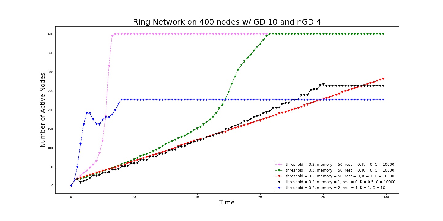
Spread of the signal as a function of active neurons.

Run a full scale experiment

In order to asses global features, we run experiments for every seed node i and obtain the activation times for every neuron j i.e. create a distance matrix whose (i,j) entry is the first time the node j is activated on a contagion starting from i. Distance matrices enable a global scale TDA analysis.

FAT, CS = BN.make_distance_matrix(TIME, C, K)

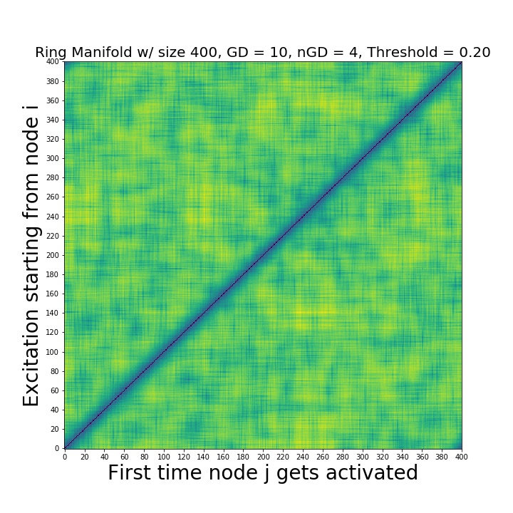
The distance matrix. The input for the persistent homology.

Persistence diagrams

Once we created the distance matrices, we can look at the topological features across different contagions and different topologies.

delta_min, delta_max = BN.compute_persistence(FAT, spy = True)##returns the lifetime difference of the longest living one cycles(delta_min) and lifetime difference of the longest and shorthest living one cycles(delta_max)

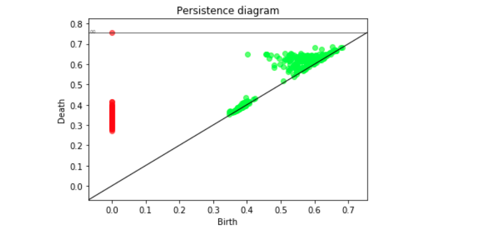
Persistence diagram computed from the distance matrix via Rips filtration. Green is 1-D features, red is 0-D features.